
It’s October already, which means we’re on a bullet train to the holiday season. But with inflation in the US currently surpassing 8 percent, it’s getting harder and more expensive to celebrate as we’ve done in years past.
But a little planning can go far. Tracking prices ahead of the big holiday sales can be incredibly helpful when it comes to getting more bang for your buck. And if you start early this year, you can even skip the lines, the rush, and any stock or supply chain problems that may arise.
Pulling all the relevant information you need from Amazon (such as price, photos, dimensions, and reviews) and plastering it onto a spreadsheet is easier than you think—you just need the correct function to do the trick for you.
Meet the ImportFromWeb function
Spreadsheet programs such as Microsoft Excel or Google Sheets have useful automated tools called functions.
But that’s just the very tip of the iceberg—spreadsheet programs can be incredibly powerful, and add-ons can make them even more impressive. Google has an entire library of optional widgets called Google Workspace Marketplace. It works just like the extension store in your browser, and you can take your pick from thousands of tools to add some oomph to the programs you use daily.
[Related: 3 spreadsheet tips to make beginners feel like pros]
The ImportFromWeb function is one of them. This add-on will automatically pull specific details from a webpage and copy them seamlessly onto a spreadsheet for you. It’s optimized to work with Amazon, so in one column you can just copy the URLs of the products you want to keep an eye on, and the function will display relevant information about them, like the price, the average review score, and other specs you might want to track.
Using this function, you can easily create a holiday wish list for the items you want, which will serve as a basic budget and a useful baseline parameter in case prices change.
How to use the ImportFromWeb function
As with browser extensions, start by going to the ImportFromWeb page on the Google Workspace Marketplace and installing the add-on. But unlike browser extensions, you’ll need to activate this new function to use it. To do this, open Google Sheets, go to Extensions on the main menu bar at the top of your screen, and hover over ImportFromWeb—it should be the last option on the list. Finally, in the emerging menu, click on Activate add-on. Now you’re ready to start importing data from Amazon.
Add some descriptors
Open a new spreadsheet and start by planning what information will go on each column. Use the first cell on each one to describe the column’s content, and assign the first column to the links of the products you’ll be tracking—type in Links in the first cell of the first column. This is going to be row number 1, and it’ll be important later.
Continue by assigning descriptors to each column. If you’ve ever used a function in a spreadsheet, you’ll know that you need to give the tool some parameters so it can understand what to fetch specifically, and from where. ImportFromWeb is no exception, and to use it, you’ll need descriptors that tell it exactly what you want to copy from an Amazon product page. If you’re budgeting for the holidays, the most relevant descriptors for you might be an item’s name, price, review score, and image.
ImportFromWeb has all these descriptors, but you’ll need to use the correct names for them, which you’ll type in the first row of each column. A product name is called title, while the price is sale_price, or list_price, if you want to know the original amount the manufacturer priced the item for.
This all sounds like a lot, but don’t worry: the developers of the add-on created a handy selector library for Amazon web pages you can consult at any time. (They also have a similar resource for Yahoo! Finance, if that’s something you’re into.) You can use as many descriptors as you want, but remember that the more you add, the harder your spreadsheet will be to navigate, as it’ll have more columns.
Gather your links
In your first column, under Links, paste the URLs of the products you want to track. There should be one in each cell. Keep in mind that you don’t have to have a full list right away—you can start with one and then automatically replicate the formula as you add more links to the list. Don’t worry, we’ll have more on that later.
Type in your formula
To quote artists from the early 00’s series MTV Cribs, this is where the magic happens. Paste an Amazon product link in your first column, and on the cell to the right, summon the ImportFromWeb function by typing =Importfromweb. (Pro tip: As you type, Google Sheets will show you the available functions in a pop-up menu, so you can navigate that instead of actually finishing typing.)
Your formula will need two parameters, and the first one tells the function where to go to fetch the information you need. For this, you will use the coordinates of the cell where you pasted your first Amazon product link—in this case, I used A3.
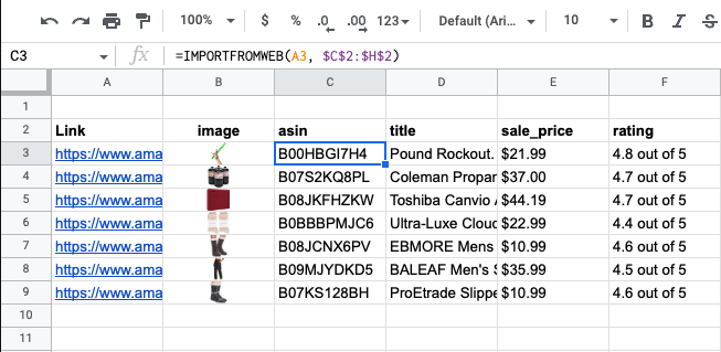
Separate the parameter with a comma, and type in the coordinates of the cells where you want the data to display. You can add these coordinates one by one, but using a range is easier. For that, type in the coordinate for the first cell in the range, and after a colon, type the coordinate of the last cell in the range. For example, if your descriptors go from columns C to H, you’ll type C2:H2.
Notice how we used C2 instead of C3, which is the actual coordinate of the highlighted cell in the image above. This is because your descriptor row is officially row number 1 (we told you that detail would be important later). You can save yourself some confusion if you, unlike the example above, use the first row in the spreadsheet as your descriptor row. Still, it’s useful to know how this all works if, for whatever reason, you want to start your table further down.
Finish setting up your formula by closing the parentheses and hitting Enter or Return on your keyboard. In a moment, you’ll see data magically appearing in your spreadsheet. Congratulations—you’ve got your first row of data lined up and ready! Give yourself a pat on the back. You’re doing great.
Paste and replicate ad infinitum
If you know anything about spreadsheet formulas, you’ll notice that the one we used above is a little bit limited, meaning it will only work for one URL and one specific range of cells, forcing you to do this whole process all over again for each product you want to track. Gross.
Technically, this limitation is true, but there’s an easy workaround—type dollar signs before each character of the coordinates determining the range of cells where you want the data to display, and the formula will work with any other web page address you paste under the first one. Following the previous example, your coordinates will go from C2:H2 to $C$2:$H$2.
Now, paste more URLs in your Link column, and then click on the cell where the formula is—the one to the right of the first link. You’ll notice a blue outline appears around the cell with a blue square in the bottom right corner of it. Click that square and drag it down so that it extends down the column to the length of your list of links. Wait a couple of seconds and voilá—you’ve got data.
Bonus: Add a product image
If you’re more of a visual person, it’s likely that the name of an Amazon product doesn’t tell you much. But spreadsheets are mighty tools, so if you need a photo, there’s a built-in function that can display a product’s image in its own column when you use it along with ImportFromWeb.
First, make sure that one of the descriptors you used when setting up your spreadsheet was featured_image_source. This will tell the function to fetch the URL for the main photo Amazon uses to promote a product. In a new column, summon the IMAGE function by typing =Image, and then use the coordinate of the cell displaying the image URL as a parameter. Close the parentheses, hit Enter or Return, and see the photo appear.
Troubleshooting
There’s a chance you might encounter a few glitches when using the ImportFromWeb function. You’ll see if this is the case if your cells populate with ugly #SELECTOR_RETURNS_NULL notices.
Most of these problems happen when you don’t use the correct Amazon URL. ImportFromWeb needs a specific product page to work properly, and as you might have noticed from browsing this massive marketplace, sometimes prices change depending on the specific model or size of a product. Book pages, for example, often require users to choose from paperback, hardcover, or Kindle options to provide a final price. Something similar happens with shoes, where some specific colors may be on sale, but others might be at full price. Going back to Amazon and making these choices before you copy and paste the URL in your spreadsheet will solve most of these problems.
[Related: 5 tips for tracking out-of-stock items this holiday season]
You might see the same error when using the correct product pages, but that just might be an error on the back end of the Amazon page. Unfortunately, if that is the case, there’s nothing you can do to fix it.
If you see an #EVALUATION_FAILED or #ERROR_IN_SELECTORS notice, that means there’s something wrong with the formula you’re using. Go back, look at it carefully, and make sure the parameters you used are correct and that you altered the formula so it works with links in other cells.
As you paste more links to your spreadsheet, you can just select the last cell in the formula column and drag the blue square to tell ImportFromWeb to go fetch the corresponding data for that new item on your list. Use this file as a baseline and don’t forget to complement your holiday shopping strategy with other methods to track down sales and hard-to-find products. Happy savings!